Supervised Algorithms

Machine learning: Supervised learning.

Currently, lots of people talk about machine learning and its applications. People consider that the success of companies rests in the opportunity of applying ML techniques in your business. In this way, it is important having some knowledge about these techniques and more importantly how to use these techniques.

The idea of this project is to show some of the techniques available in machine learning, and we are going to start with one of the big branches: supervised learning methodologies. Supervised learning scenario occurs when “a set of variables that might be denoted as inputs have some influence on one or more outputs” (Hastie, Tibshirani, and Friedman, 2009). The purpose of supervised learning is to use the inputs to predict the values of the outputs.

On the other hand, depending on the characteristic of the output, we have different problems. If the output is a quantitative variable, we have a regression problem. In case that the output is qualitative, we have a classification problem. However, in the case of some qualitative outcomes with two classes, we can use regression techniques into classification problems.

Classification

The focus of the section is to consider the classification problem, then compare some techniques in one simple exercise and finally to use a cross-validation method for estimating the prediction error. All these steps are made in R program using the following libraries:

library(tidyverse)    #ggplot
library(kknn)         #kknn
library(e1071)        #svm
library(rpart)        #tree
library(randomForest) #RF
library(ada)          #Boost
library(caret)        #CV

Using the purchasedBikes file, this table contains 1000 observations of 12 variables. We want to use 11 predictor variables for predict the binary class as output PurchasedBike. It indicates if a customer bought or not a bicycle.

purchased_bike <- read.table("purchasedBikes.csv",
                              header = TRUE,
                              sep = ";",
                              dec = ",",
                              row.names = 1)

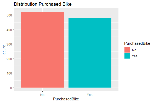
Because the purpose of this exercise is to compare the performance of some techniques, we can see that the outcome variable PurchasedBike is well balanced (48% of the observations in the data set corresponding to Yes value).

ggplot(data = purchased_bike) +
  geom_bar(aes( x = PurchasedBike, fill = PurchasedBike)) +
    labs(title = "Distribution Purchased Bike")  

The goal of this exercise is to compare several classification techniques with this example table. Here, the purpose is to predict Yes value in the PurchasedBike using ten cross-validations with 5 groups with the methods:

• Support Vector Machine
• KNN
• Bayes
• Decision tree
• Random Forest
• Boosting methods (AdaBoost)

Furthermore, the two metrics that we are going to use for determining how good our model is are:

• How many “yes” purchase bike variable the model detects. High values are best.
• Minimum average global error, calculated as 1 - accuracy, where accuracy is calculated as the number of correct predictions divided by the number of total predictions. Low values are best.

For determining the number of “yes” in the PurchasedBike and the average global error, we do the following code:

#Number of observation
n <- dim(purchased_bike)[1]

#SVM
yes_detect_svm   <- rep(0,10)
error_detect_svm <- rep(0,10)

#KNN
yes_detect_knn   <- rep(0,10)
error_detect_knn <- rep(0,10)

#Bayes
yes_detect_bayes   <- rep(0,10)
error_detect_bayes <- rep(0,10)

#trees
yes_detect_tree   <- rep(0,10)
error_detect_tree <- rep(0,10)

#RFs
yes_detect_RF   <- rep(0,10)
error_detect_RF <- rep(0,10)

#boosting
yes_detect_boosting   <- rep(0,10)
error_detect_boosting <- rep(0,10)

# cross validation 10 times
for(i in 1:10) {  #10
  groups <- createFolds(1:n,5) #5 groups

  #SVM
  yes_svm   <- 0
  error_svm <- 0

  #KNN
  yes_knn   <- 0
  error_knn <- 0

  #Bayes
  yes_bayes   <- 0
  error_bayes <- 0

  #trees
  yes_tree   <- 0
  error_tree <- 0

  #RFs
  yes_RF   <- 0
  error_RF <- 0

  #boosting
  yes_boosting   <- 0
  error_boosting <- 0

  # This for does "cross-validation"  with 5 groups (Folds)
  for(k in 1:5) {   #5

    training  <- groups[[k]]              #list
    ttesting  <- purchased_bike[training,]
    tlearning <- purchased_bike[-training,]

    #SVM
    model      <- svm(PurchasedBike~., data = tlearning, kernel ="radial")
    prediction <- predict(model, ttesting)
    Actual     <- ttesting[, 12]
    MC         <- table(Actual, prediction)

    # "Yes" purchase detection
    yes_svm <- yes_svm + MC[2,2]
    # Error detection
    error_svm <- error_svm + (1 - (sum(diag(MC)))/sum(MC))*100

    #KNN
    model      <- train.kknn(PurchasedBike~., data = tlearning, kmax = 7)
    prediction <- predict(model,ttesting[, -12])
    Actual     <- ttesting[, 12]
    MC         <- table(Actual, prediction)

    # "Yes" purchase detection
    yes_knn <- yes_knn + MC[2,2]
    # Error detection
    error_knn <- error_knn + (1 - (sum(diag(MC)))/sum(MC))*100

    #Bayes
    model      <- naiveBayes(PurchasedBike~., data = tlearning)
    prediction <- predict(model, ttesting[,-12])
    Actual     <- ttesting[,12]
    MC         <- table(Actual, prediction)

    # "Yes" purchase detection
    yes_bayes <- yes_bayes + MC[2,2]
    # Error detection
    error_bayes <- error_bayes + (1 - (sum(diag(MC)))/sum(MC))*100

    #trees
    model      <- rpart(PurchasedBike~. ,data = tlearning)
    prediction <- predict(model, ttesting, type='class')
    Actual     <- ttesting[, 12]
    MC         <- table(Actual, prediction)

    # "Yes" purchase detection
    yes_tree <- yes_tree + MC[2,2]
    # Error detection
    error_tree <- error_tree + (1 - (sum(diag(MC)))/sum(MC))*100

    #RFs
    model      <- randomForest(PurchasedBike~., data = tlearning, importance=TRUE)
    prediction <- predict(model, ttesting[, -12])
    Actual     <- ttesting[, 12]
    MC         <- table(Actual, prediction)

    # "Yes" purchase detection
    yes_RF <- yes_RF + MC[2,2]
    # Error detection
    error_RF <- error_RF + (1 - (sum(diag(MC)))/sum(MC))*100

    #boosting
    model      <- ada(PurchasedBike~., data = tlearning, iter=20, nu = 1, type = "discrete")
    prediction <- predict(model, ttesting[, -12])
    Actual     <- ttesting[, 12]
    MC         <- table(Actual, prediction)

    # "Yes" purchase detection
    yes_boosting <- yes_boosting + MC[2,2]
    # Error detection
    error_boosting <- error_boosting + (1-(sum(diag(MC)))/sum(MC))*100

  }

  #SVM  
  yes_detect_svm[i]   <- yes_svm
  error_detect_svm[i] <- error_svm/5

  #KNN
  yes_detect_knn[i]   <- yes_knn
  error_detect_knn[i] <- error_knn/5

  #Bayes
  yes_detect_bayes[i]   <- yes_bayes
  error_detect_bayes[i] <- error_bayes/5

  #trees
  yes_detect_tree[i]   <- yes_tree
  error_detect_tree[i] <- error_tree/5

  #RF
  yes_detect_RF[i]   <- yes_RF
  error_detect_RF[i] <- error_RF/5

  #boosting
  yes_detect_boosting[i]   <- yes_boosting
  error_detect_boosting[i] <- error_boosting/5
}

Finally, we create three auxiliary tables for showing the results:

colors <- c("SVM"      = "blue",
            "KNN"      = "red",
            "Bayes"    =  "orange",
            "Tree"     = "purple",
            "RF"       = "black",
            "Boost" = "green"
)

detect <- tibble(Iteration = seq(1,10),
                 SVM = yes_detect_svm,
                 KNN = yes_detect_knn,
                 Bayes = yes_detect_bayes,
                 Tree = yes_detect_tree,
                 RF   = yes_detect_RF,
                 Boost = yes_detect_boosting)

global_error <- tibble(Iteration = seq(1,10),
                 SVM = error_detect_svm,
                 KNN = error_detect_knn,
                 Bayes = error_detect_bayes,
                 Tree = error_detect_tree,
                 RF   = error_detect_RF,
                 Boost = error_detect_boosting)

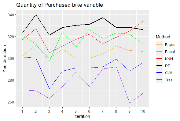
The plot with the yes value detection shows us that the method random forest has on average the best capacity for detecting the positive cases of bikes purchased.

ggplot(data = detect, aes(x = Iteration) ) +
  geom_line(aes( y = SVM, color = "SVM") ) +
  geom_line(aes( y = KNN, color = "KNN")) +
  geom_line(aes( y = Bayes, color = "Bayes")) +
  geom_line(aes( y = Tree, color = "Tree")) +
  geom_line(aes( y = RF, color = "RF"), size = 1) +
  geom_line(aes( y = Boost, color = "Boost")) +
  scale_x_continuous(breaks=c(1:10), labels=c(1:10),limits=c(1,10)) +
  labs(x = "Iteration",
       y = "Yes detection",
       color = "Method",
       title = "Quantity of Purchased bike variable"
       ) +
  scale_color_manual(values = colors)

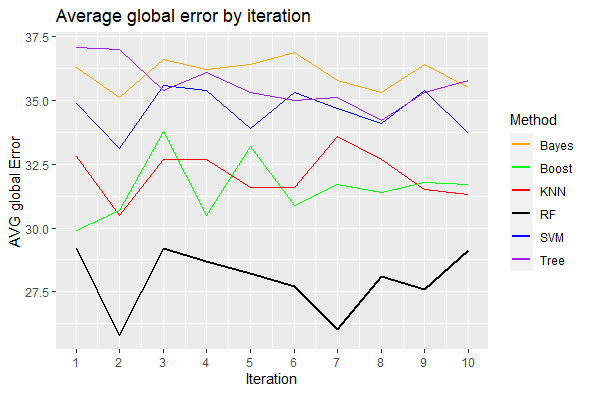
Besides, Random forest also has the lest average global error, so this method also classifies very well the negative case of bike did not purchase.

ggplot(data = global_error, aes(x = Iteration) ) +
  geom_line(aes( y = SVM, color = "SVM") ) +
  geom_line(aes( y = KNN, color = "KNN")) +
  geom_line(aes( y = Bayes, color = "Bayes")) +
  geom_line(aes( y = Tree, color = "Tree")) +
  geom_line(aes( y = RF, color = "RF"), size = 1) +
  geom_line(aes( y = Boost, color = "Boost")) +
  scale_x_continuous(breaks=c(1:10), labels=c(1:10),limits=c(1,10)) +
  labs(x = "Iteration",
       y = "AVG global Error",
       color = "Method",
       title = "Average global error by iteration"
  ) +
  scale_color_manual(values = colors)

References

Hastie T., Tibshirani R., Friedman J. 2008. The elements of Statistical Learning. Springer.